Housing

class: center, middle, inverse, title-slide

.title[
# Housing
]
.subtitle[
## Set 10
]
.author[
### Andrew Dickinson
]
.date[
### Fall 2022
]

---

class: inverse, middle
# Content

.hi-white[(i) Homeownership]

.hi-white[(ii) Rental markets]

---
# Housekeeping

.pull-left[
.hi[PS03] _(due Friday, Nov. 25)_
- Posted now (a couple of minutes ago)
]

.pull-right[
.hi[PS04] _(due Wed, Nov. 30)_
- will be posted by Mon next week
]

.hi[TotC book report] _(due Thu, Dec. 8)_
- Short (1000 words) assignment 
- rubric posted on canvas and on the course repo
- will be checking for plagiarism

.hi-red[Final] _(14:45 Wed, Dec. 7)_
- [final schedule](https://registrar.uoregon.edu/calendars/examinations)
- Comprehensive exam with an emphasis on the newer material

---
class: inverse, middle
# Housing markets

---
# Housing markets

Distinguish the following two markets:
- .hi[Rental Market:] Supply and Demand for rentals
- .hii[Housing Market:] Supply and Demand for houses

<br>

_Why is it important to distinguish these?_
 - A house is an asset. A month of rent is not
 - Homeowners are much less mobile than renters
  
  
---
# Homeownership

Following the great depression the .hi[New Deal] stimulated private homeownership by making it easier for individuals to buy and sell houses
- established the .hi[Federal Housing Administration] and the .hi[Home Owners Loan Corporation]

The Federal Government .hi[invented] the modern home mortgage by .hii[insuring] private home loans

Which .hi[incentivised] banks to accept:
- .hi-red[smaller] down payments
- .hi-red[lower] interest rates
- .hi-blue[longer] term loans (15/30 year mortgage)

Allowed citizens to buy homes that they otherwise would not have afforded, establishing cycles of .hi[generational wealth]

---
# Homeownership

_Why is buying a home different than buying a pair of jeans?_

Houses are a major investment and store of value (.hi[equity])

Homeownership remains a .hi[key] component of household wealth
- The value is subject to some uncertainty
 
--

<br>
 
Purchasing a home is a .hi[dynamic] (forward-looking) decision

Jeans (a pure consumption good) is not really a store of value

We will focus on the rental  market.
--
 But first some data.

---
class: clear
# Rentals vs Homeowners

.center[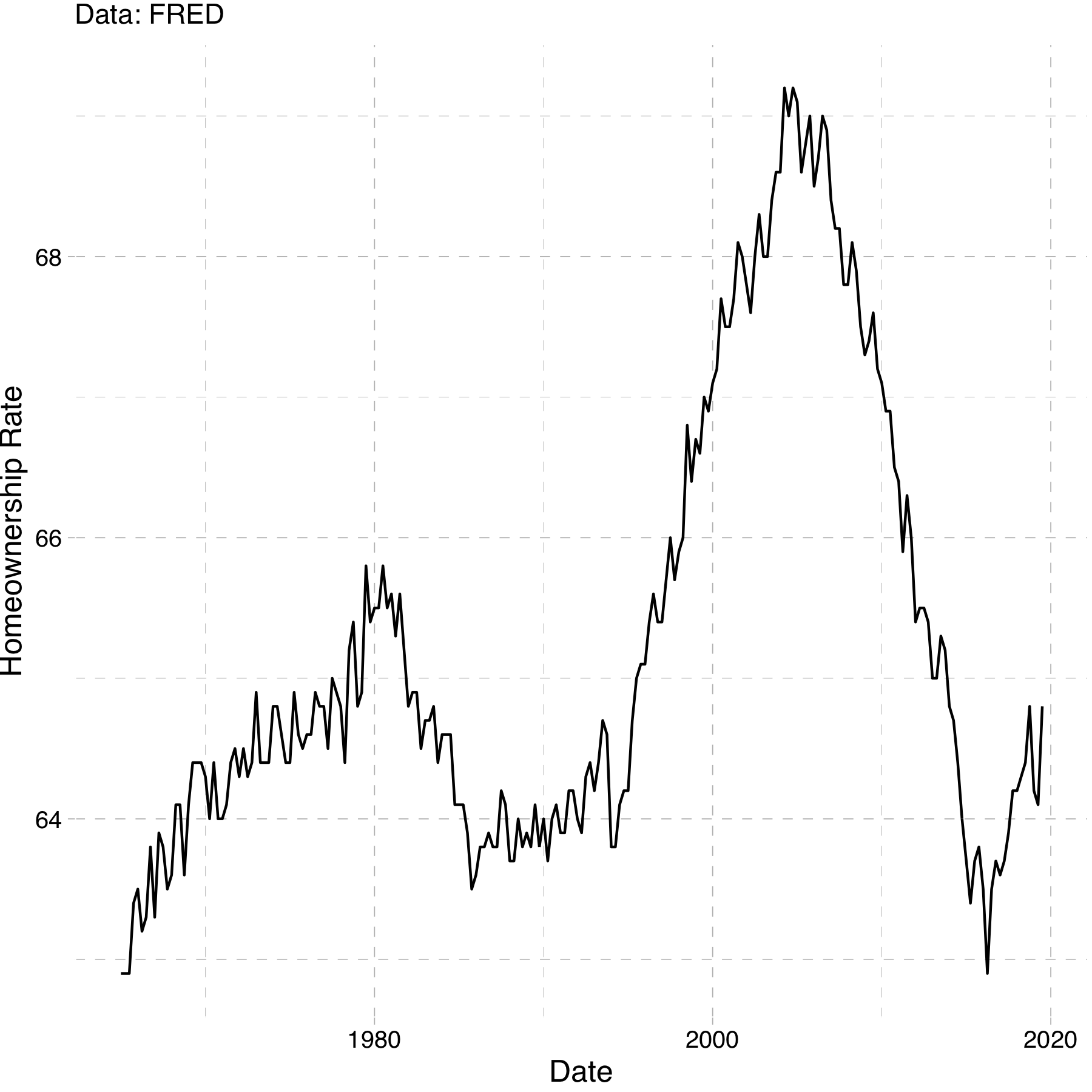
![:scale 60%](figures/ownership_plot.png)
]

.smallerer[Why such a big spike?]

---
# Housing prices (nominal)

.center[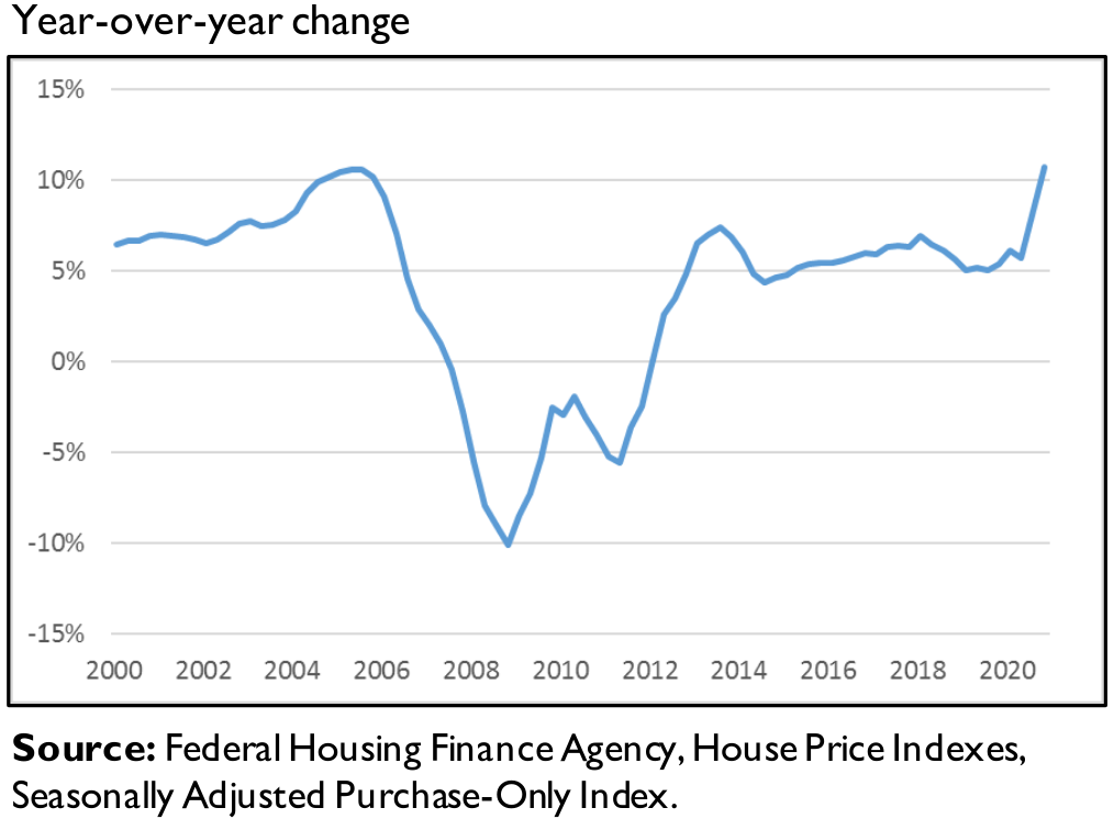
![:scale 80%](./figures/nominal-prices.png)
]

---
# Housing inventory

.center[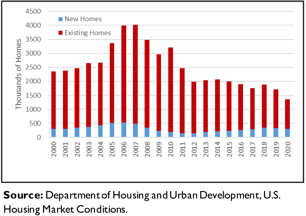
![:scale 80%](./figures/inventory.png)
]

---
# Housing crisis (summarized)

.center[.hi[What caused the housing market crash in 2007?]]

.center[.hii[Among many other things, subprime mortgages]]

Historically, mortgage loans were a safe investment as defaulting was rare

Mortgages are typically bundled together with lots of other home loans and sold on a marketplace better banks

Due to growing home prices in the US housing market, these ".hi[securities]" were desirable and had higher returns than US treasury bonds and were in high demand. Lenders tried to keep up.

Mortgage lenders took too much risk by extending loans the millions of Americans who could not afford them

---
# Housing crisis (summarized)

These high risk, subprime loans were bundled into .hi[securities] with lower risk loans and sold them to banks

Rating agencies didn't fully understand the extent to which lenders were extending subprime loans and granted high grades (AAA)

Then the housing bubble popped, and high interest rates set in on adjustable loans, massive amounts of people defaulted

People shorted the banks on their investments and it lead to a massive financial crisis

---
class: inverse, middle 
# Rental markets

---
# Rental market model

Just like labor markets, each city has its own market for rental units 
- Consists of suppliers (absentee landlords) 
- Individuals making optimal housing demand decisions

.hi[Important:] Firms (landlords) supply housing to households

.hi[Assumptions:]

.hii[(i)] No individual landlord can influence the price of rents

.hii[(ii)] Landlords decide how much housing to provide

.hii[(iii)] The amount of housing they provide will again come from profit maximization

---
# Rental market model: Perf Comp

Profit function given by:

`\begin{align*}
\pi(Q) = P*Q - TC(Q)
\end{align*}`

.hi[Note:] Now cost is a function of quantity

Implicitly we are assuming that at any quantity, the firm will use the optimal level of labor and capital

Marginal profit equals zero , `\(\frac{\Delta \pi(Q)}{\Delta Q}= 0\)`:

`\begin{align*}
 \frac{P*\Delta Q}{\Delta Q} - \frac{\Delta TC(Q)}{\Delta Q} = 0
\end{align*}`

---
count: false
# Rental market model: Perf Comp

Profit function given by:

`\begin{align*}
\pi(Q) = P*Q - TC(Q)
\end{align*}`

.hi[Note:] Now cost is a function of quantity

Implicitly we are assuming that at any quantity, the firm will use the optimal level of labor and capital

Marginal profit equals zero , `\(\frac{\Delta \pi(Q)}{\Delta Q}= 0\)`:

`\begin{align*}
 \frac{P*\Delta Q}{\Delta Q} - \frac{\Delta TC(Q)}{\Delta Q} &= 0\\
 P &= \frac{\Delta TC(Q)}{\Delta Q}
\end{align*}`

---
count: false
# Rental market model: Perf Comp

Profit function given by:

`\begin{align*}
\pi(Q) = P*Q - TC(Q)
\end{align*}`

.hi[Note:] Now cost is a function of quantity

Implicitly we are assuming that at any quantity, the firm will use the optimal level of labor and capital

Marginal profit equals zero , `\(\frac{\Delta \pi(Q)}{\Delta Q}= 0\)`:

`\begin{align*}
 \frac{P*\Delta Q}{\Delta Q} - \frac{\Delta TC(Q)}{\Delta Q} &= 0\\
 P &= \frac{\Delta TC(Q)}{\Delta Q}\\
 P &= MC(Q)
\end{align*}`

---
count: false
# Rental market model: Perf Comp

Profit function given by:

`\begin{align*}
\pi(Q) = P*Q - TC(Q)
\end{align*}`

.hi[Note:] Now cost is a function of quantity

Implicitly we are assuming that at any quantity, the firm will use the optimal level of labor and capital

Marginal profit equals zero , `\(\frac{\Delta \pi(Q)}{\Delta Q}= 0\)`:

`\begin{align*}
 \frac{P*\Delta Q}{\Delta Q} - \frac{\Delta TC(Q)}{\Delta Q} &= 0\\
 P &= \frac{\Delta TC(Q)}{\Delta Q}\\
 P &= MC(Q)
\end{align*}`

.center[.hi[Increasing marginal costs leads to upward sloping supply curves!]]

---
class: inverse, middle

# Monopoly

---
# Rental market model: Monopoly

Now let's consider the .hi[monopoly] situation:

.hi[Assume:]

.hii[(i)] One seller of the good (rental units)

.hii[(ii)] The monopolist has market power; ability to set prices

.hii[(iii)] The monopolist is a profit maximizer

---
# Rental market model: Monopoly

Equilibrium relies on the assumption that firms maximize profits

Now TR is a function of quantity

`\begin{equation*}
TR = P(Q)*Q
\end{equation*}`

Quantity of houses that the monopolist produces changes the market price

`\(P(Q)\)` in this context is called the inverse demand function
  
--

.hi[Profit is given by:]

`\begin{align*}
\pi(Q) = P(Q)*Q - TC(Q)
\end{align*}`

---
# Rental market model: Monopoly

Profit Maximization gives us the familiar `\(\frac{\Delta \pi(Q)}{\Delta Q} = 0\)`

`\begin{align*}
\frac{\Delta P(Q)*Q}{\Delta Q} - \frac{\Delta TC(Q)}{\Delta Q} = 0 
\end{align*}`
  
---
count: false
# Rental market model: Monopoly

Profit Maximization gives us the familiar `\(\frac{\Delta \pi(Q)}{\Delta Q} = 0\)`

`\begin{align*}
\frac{\Delta P(Q)*Q}{\Delta Q} - \frac{\Delta TC(Q)}{\Delta Q} &= 0 \\
MR(Q) &= MC(Q)
\end{align*}`

.hi[Note:] Now, `\(\frac{\Delta P(Q)*Q}{\Delta Q} \neq P\)`.

---
# Simple monopoly example

---
# Monopoly Graph

---
count: false
# Monopoly Graph

---
count: false
# Monopoly Graph

---
class: inverse, middle
# Rental markets across cities

---
# Rents across cities

.hi[Key question:] What causes rental curves to vary across cities?

--
  
Supply curves across cities are impacted by:
- .hi-blue[local construction costs]
- .hi-green[limited land availability] (for development)
- .hi-green[land-use regulations]

.hi-blue[Local construction costs]: shifts supply curve (labor is more expensive for all firms in one area vs another)

.hi-green[Land availability] + .hi-green[land use regulations:] rotates supply curve (changes in the marginal cost of developing land)

---
# Rents across cities

_Why do changes in local constructions costs shift the supply curve when land use regulations rotate it?_

.hi[Answer:]

Changes in .hi-blue[construction costs] impact all development equally.
- if wood becomes more expensive then every project becomes equally more expensive across the city

Changes in .hi-green[land availability] or .hi-green[land-use regulations] increase the .hii[opportunity cost] of developing additional plots of land
- prices bid faster for each additional development

---
# Urban Housing Supply Curves

---
count: false
# Urban Housing Supply Curves

.hii[purple:] lower construction cost (lower intercept)

---
count: false
# Urban Housing Supply Curves

.hi-green[green:] higher .green[land-use regulations]

---
class: inverse, middle
# Rent control

---
# Rent control

.hi[Definition:] .hii[Rent Control]

> A _price ceiling_ set on rental units

> _Price Ceiling:_ Max allowed price on the market

Brief History (US):

- Started around WW1. Expanded during WWII
  
--

- 1970: Nixon puts 90-day freeze on prices to combat inflation

- _Mostly_ a .hi[place based policy]. 
  - SF, NY, LA, Oakland, DC, Berkeley, West Hollywood
  - Oregon: first state to have  state-wide rent control

---
class: clear
# Rent Control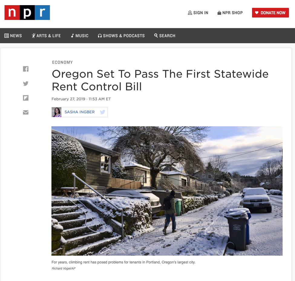

![](figures/oregon_control.png)

---
# Rent Control in Oregon

### Senate Bill 608

2019: Oregon passes .hi[state-wide] rent control 
- limits annual increases to inflation (2-3%) + 7%
- landlords can increase rent without limit for new tenants

Also includes a series of eviction protections for renters

---
class: inverse, middle
# Land use restrictions

---
# Land use restrictions

Land use restrictions limit what one can do with available land.

Examples:

.hi[(i)] Density restrictions

.hi[(ii)] Minimum lot sizes

.hi[(iii)] Parking requirements

.hi[(iv)] Sidewalk and street size requirements

.hi[(v)] Height restrictions

Not all of these are bad things. But they do make developing land more expensive.

---
# Wharton Index

![](figures/wharton_new.png)

Higher values of the Wharton index `\(\implies\)` tighter land use restrictions

---
# Example

---

# A Model

Do Land-Use regs and rent control interact? Absolutely! Let's model it

`\begin{align*}
P(Q_d) &= 20 - 2*Q_d\\
P(Q_s) &= 8 + Q_s\\
\end{align*}`

Compute the equilibrium. Graph it, if that is helpful

- Now suppose the government ratchets up land-use regs. New supply is given by:

`\begin{align*}
P(Q_s^{new}) = 8 + 2*Q_s^{new}
\end{align*}`

---
# Example

Old eq: `\(Q^* = 4\)`, `\(P^* = 12\)`

New eq: `\(Q^* = 3\)`, `\(P^* = 15\)`

Government comes in and says the rents are too high. Rent control set at `\(12\)` per unit. Now you have:

`\begin{align*}
12 = 8+2*Q_s \implies Q_s = 2
\end{align*}`

---
count: false
# Example

Old eq: `\(Q^* = 4\)`, `\(P^* = 12\)`

New eq: `\(Q^* = 3\)`, `\(P^* = 15\)`

Government comes in and says the rents are too high. Rent control set at `\(12\)` per unit. Now you have:

`\begin{align*}
12 = 8+2*Q_s &\implies Q_s = 2\\
12 = 20 - 2*Q_d &\implies Q_d = 4
\end{align*}`

---
count: false
# Example

Old eq: `\(Q^* = 4\)`, `\(P^* = 12\)`

New eq: `\(Q^* = 3\)`, `\(P^* = 15\)`

Government comes in and says the rents are too high. Rent control set at `\(12\)` per unit. Now you have:

`\begin{align*}
12 = 8+2*Q_s &\implies Q_s = 2\\
12 = 20 - 2*Q_d &\implies Q_d = 4
\end{align*}`

So we have a .pink[shortage] of two units at the .hi.purple[old] equilibrium price. 😧

---
# A Note

We wont have time (but it might be good practice) for you to think through what would happen if the market was a .hi[monopoly]
- Similar to the .hi.purple[monopsonist], rent control can actually .pink[lower prices] in a completely .purple[monopolized] housing market

Let's take a (quick) look at some recent empirical evidence

---
# Empirics

[Diamond et. al (2019)](https://web.stanford.edu/~diamondr/DMQ.pdf)
- 1979: Rent control in SF put in place for all standing buildings with 5 apartments or more
- New buildings exempt (to promote developers to continue building)
- Small multi-family apartment buildings ("mom & pop") exempted
- 1994: Exemption for small multi-family buildings removed. All apartments .hi[built before 1980] subject to rent control
    
  
---
# Empirics

In this study:

- .hi[Treatment:] Those living in small apartment complexes (5 or less) built in 1979 or before

- .hi[Control:] Those living in small apartments complexes (5 or less) built after 1979 (not subject to rent control)

A fair comparison? Maybe concerned that those living in apartments built before or after 1979 are systematically different.

.hi.slate[Main Findings]:

.hi[(i)] Reduced renter mobility by ~20%

.hi[(ii)] Reduced housing supply by about 15%