class: center, middle, inverse, title-slide # Econ 330: Urban Economics ## Lecture 12 ### Andrew Dickinson ### 06 December, 2021 --- class: inverse, center, middle # Lecture 12: The Geography of Income Inequality^{.smallest[.hii[†]]} .footnote[.hii[†] This lecture uses content from Raj Chetty's course: https://opportunityinsights.org/course/ ] --- class: inverse, middle # Schedule .pull-left[ - .hi-white[The rise of "big data"] - .hi-white[The American Dream] - .hi-white[The causal effect of neighborhoods] - .hi-white[Geography of upward mobility] ] .pull-right[ .ul[.hi-white[Upcoming]] - .hi-white[PS03 due tonight] - .hi-white[PS04 due Tuesday at 4pm] - .hi-white[Final Wednesday at 8am] ] --- class: inverse, middle # The rise of "big data" --- # Theoretical social science Until very recently, social scientist were very limited by data to study these types of .hi[policy questions] Social science has been mostly a .hii[theoretical field] to make policy recommendations -- - Develop mathematical models (economics) - Qualitative theories (sociology) -- .hi[Problem:] We were never able to test most of these theories - Led to politicization of scientific questions such as > Is Obamacare reducing job growth in America? --- # Big data and empirics Social sciences are more empirical thanks to growing availability of data - Test and improve theories using real world data -- .center[ 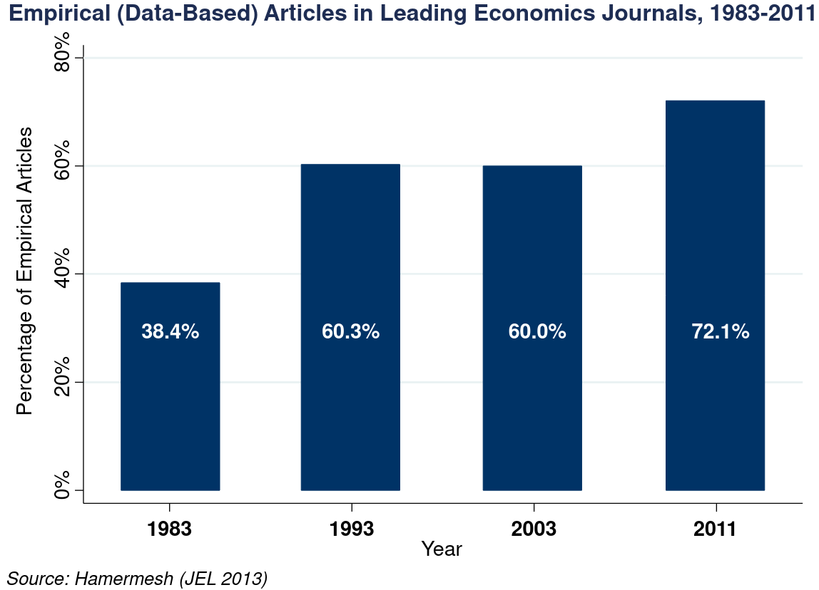 ] --- # Big data and empirics .pull-left[ What is .hi[_"Big data"_]? > Large datasets ] -- .pull-right[ Where did .hi[_"Big data"_] come from? Product of the .hii[internet age] - Information costs `\(\rightarrow 0\)` ] -- Product of post-internet private sector: ["Data is the new oil"](https://www.economist.com/leaders/2017/05/06/the-worlds-most-valuable-resource-is-no-longer-oil-but-data)^{.smallest[.hii[†]]} .footnote[.hii[†] Whatsapp, Robinhood] .center[  ] --- # Big data and empirics .hii[Examples:] -- .pull-left[ - Government data: Tax records - Corporate data: Google etc. - Text data: Twitter, newspapers ] .pull-right[ - Satellite imagery - Cellphone location data - GitHub data ] -- .hi[Benefits:] .pull-left[ - More reliable than surveys - New variables (eg emotions, locations)] .pull-right[ - Rich coverage `\(\Rightarrow\)` study subgroups - Large samples] --- class: inverse, middle # "Big data" and the American Dream --- # The American Dream The .hi[American Dream] is an multi-faceted, abstract concept that may be interpreted in many ways -- .center[.hi[Is the American Dream alive and well today?] .hii[How should we judge that?]] -- How can we distill the concept of an the American Dream into a .hi[statistic] that we can .hii[systematically measure using big data]? -- Obama (2014): > People's frustrations are partly rooted "in the fear that their kids won't be better off than they were." -- .hi[One systematic measure the American Dream:] What fraction of children earn more income than their parents? .hii[Is this a fair measure?] -- .center[.hii[How has this statistic changed over time]] --- # Measuring the American Dream .hi[Central policy question:] Why are children's chances of climbing the income ladder falling in America? - What can we do to reverse this trend? -- Difficult to answer using .hi[historical data] and .hii[macroeconomic trends] -- .hi[Problem:] We have too few data points to test all alternative explanations -- - We never had the data to link parental income across generations --- # Measuring the American Dream Now, economists are able to observe .hi[tax records] over time; linking generational income - Chetty et al. (2017) Linking yearly reported income over time, these data can track earnings over someone's life at the .hi[individual level] -- Fine .hii[resolution] of these data provide far more information than any macro time series -- .hi[Allow researchers to observe generational differences in income] --- # The American Dream .center[ 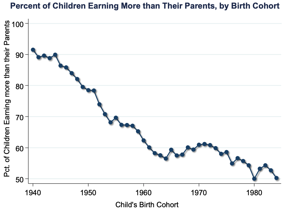 ] --- # The American Dream .center[ 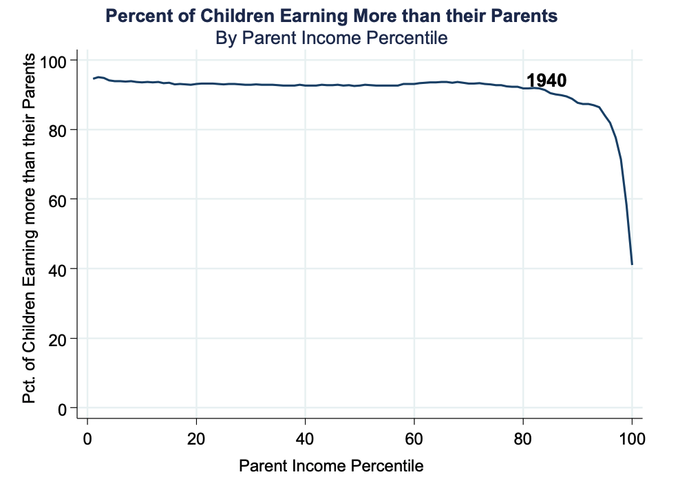 ] --- count: false # The American Dream .center[ 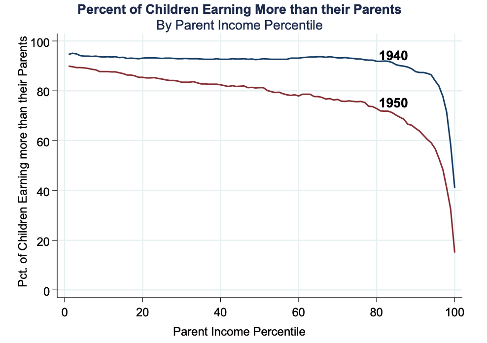 ] --- count: false # The American Dream .center[  ] --- count: false # The American Dream .center[  ] --- count: false # The American Dream .center[  ] --- # The American Dream .center[  ] --- count: false # The American Dream .center[  ] --- # The fading American Dream .center[.hi[What do these figures indicate about the American Dream?]] -- .center[.hii[It has become harder and harder to reach it]] -- <br> .hi[Two] major changes in the American economy since the 1940s: .hii[(i).] Lower total economic growth .hii[(ii).] Less equal distribution of growth --- # Growth in family income The following chart compares growth in real mean family income by quintile between 1947-1973 and 1973-2013 .center[  ] --- # Growth in family income  --- # Growth in family income .center[  ] --- # Growth in family income .hi[Two] major changes in the American economy since the 1940s: - Lower total economic growth - Less equal distribution of growth -- .hi[What policies can increase absolute mobility?] -- Consider two hypothetical scenarios for children born in 1980: .hii[(i).] .hi[Higher growth] > 1940 cohort growth rate with the 1980 cohort historical distribution .hii[(ii).] .hi[More broadly shared growth] > Same 1980 cohort historical growth rates but 1940 cohort distribution across income groups --- class: inverse, middle # Which over these scenarios would have lead to a stronger American Dream? --- # Hypothetical scenarios .center[  ] --- # Hypothetical scenarios .center[  ] --- # Hypothetical scenarios .center[  ] --- # Restoring the American Dream .hi[Main lesson:] Restoring the American Dream of high rates of upward mobility will require .hii[more broadly shared] economic growth - Need policies that will increase incomes throughout the distribution -- .hi[Two approaches of redistribution] .hii[(i).] .hi[Redistribution] - Piketty and Saez: Reduction in top income taxes and erosion of unions and min wage have led working-class Americans to fall behind -- .hii[(ii).] .hi[Human Capital Investment] - Goldin and Katz: race between education and technology – need education to keep pace with technological change to increase wage rates --- # Human Capital Investment .center[  ] --- count: false # Human Capital Investment .center[  ] --- count: false # Human Capital Investment .center[  ] --- # Human Capital Investment Education is not just about technical skills; social skills matter a lot too .hi[Implication:] Policies to improve such skills could range from changes in education and training to housing voucher policies -- .hi[So far] we have assumed that restoring the American dream is desirable. Is it? -- _Should the growth be shared equally?_ - e.g: Should we try to focus on policies that restore the fading American Dream? --- # The American Dream .qa[Q]: How does increasing equality of opportunity impact economic growth? -- - Difficult to measure effects on growth directly -- .hi[Solution:] Focus on a key channel that many economists believe is the primary driver of growth -- .center[.hi[innovation]] --- # Innovation .center[  ] --- # Another Question .qa[Q] Why would patent rates vary with parental income? -- .hi[(i).] .hi[Ability]: Children from high-income families have a greater ability to innovate -- .hi[(ii).] .hi[Preferences]: Lower-income children prefer less risky occupations -- .hi[(iii).].hi[Constraints]: Lower-income children have comparable talent and preferences but lack resources and or exposure --- # Innovation vs Math scores .center[  ] --- # Innovation vs Math scores .center[  ] --- # Innovation vs Math scores Not much of the gap is explained by ability -- .hi[It seems you need three things things:] - High quantitative ability - Rich parents - Exposure to other innovators -- Much of the gap is explained by _neighborhood effects_: e.g. what seems to matter for innovation is who you grow up around. --- # Map .center[  ] --- # Neighborhood effects .qa[Q]: How do we know that it truly is neighborhood effects (e.g who you grow up near) not driving this, and .hi[not] just ability sorting? -- - Chetty et al. isolate the causal impacts of neighborhoods by analyzing the propensity to patent by a narrow technology class <br> .hi[Intuition:] Genetic ability (sorting of high skilled labor) is unlikely to vary significantly across similar technology classes. --- class: inverse, middle # Causal Effect of Neighborhoods --- # Geography of upward mobility: Data .center[ 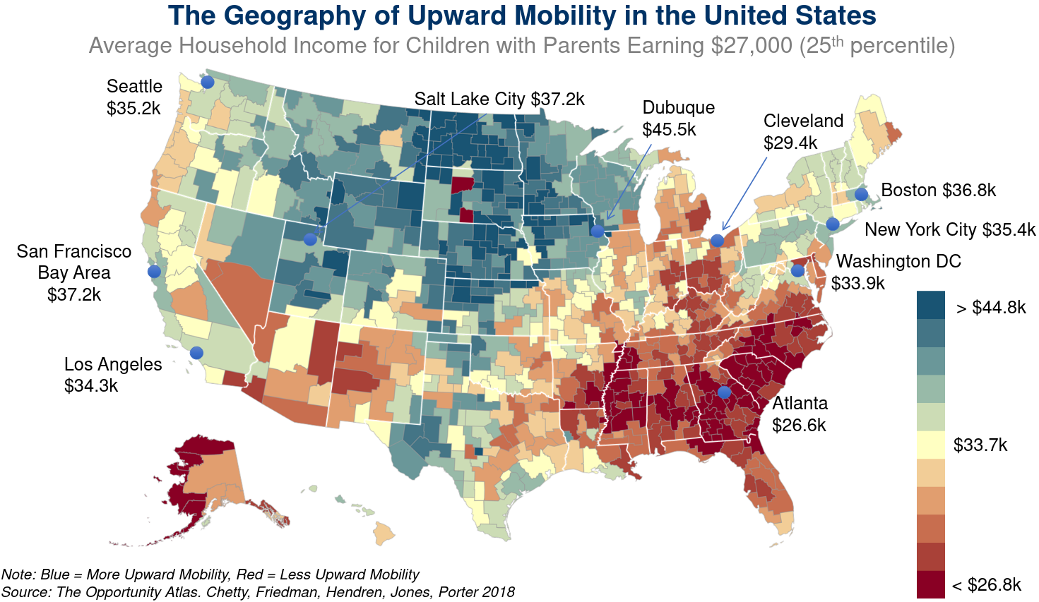 ] [Opportunity Atlas](https://www.opportunityatlas.org/) --- # Causal Effect of Neighborhoods The last topic brought rise to a bigger question: -- .center[.hi[How would we think about figuring out the impact of where a child grows up on various outcomes for the child later in life?]] -- We have two very different explanations: -- .hii[(i).] .hi[Sorting:] Similar people live near each other (educated people live near other educated people) -- .hii[(ii).] .hi[Causal impacts]: places have a .hi[causal effect] on updward mobility --- # Causal Effect of Neighborhoods What is the .hi[ideal experiment]? -- .hii[Randomly assign] children to neighborhoods. Compare adult outcome - Can't do this? So what can we do? -- .hi[Chetty & Hendren (2018)] .hi[Quasi-experiment:] Observe data on 7 million families that move .hi[Key Idea] Exploit variation in _age of child_ when family moves to identify causal impact of neighborhood environment --- # Neighborhood Effects .center[ 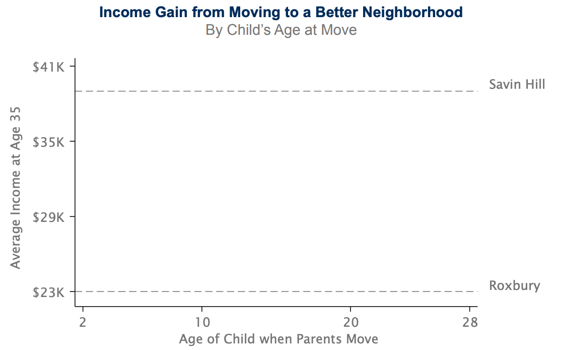 ] --- count: false # Neighborhood Effects .center[  ] --- count: false # Neighborhood Effects .center[  ] --- count: false # Neighborhood Effects .center[  ] --- # Assumptions To identify causal impact of neighborhoods, you need to believe that .hi[the timing of moves to better/worse areas are unrelated to other determinants of child's outcomes]. -- This assumption might not hold for two reasons: -- .hi[(i).] Parents who move to good areas when their children are young might be different than those who move later -- .hi[(ii).] Moving may be unrelated to other factors (e.g change in parents' job) that impact children directly -- .hi[Both of these concerns are addressed] -- - Compare across siblings --- class: inverse, middle # Geography of Upward Mobility --- # A Familiar Map  --- # Last Q OK, so: .hi[neighborhoods matter for upward mobility]. Next question: _why does this vary across cities/places?_ - To answer this question, it would be good to start by comparing places with high upward mobility to low upward mobility - Do places with higher mobility have better schools, jobs, institutions, something else? All? --- # Correlations  --- # Correlations 5 strongest correlates of upward mobility are: .hii[(i).] .hi[Segregation:] Greater racial and income segregation associated with lower levels of mobility --- count: fasle # Segregation .center[  ] --- count: fasle # Segregation .center[  ] --- count: false # Correlations 5 strongest correlates of upward mobility are: .hii[(i).] .hi[Segregation:] Greater racial and income segregation associated with lower levels of mobility .hii[(ii).] .hi[Income Inequality:] Places with a smaller middle class have less mobility -- .hii[(iii).] .hi[School Quality:] Higher expenditure, smaller classes, higher test scores `\(\implies\)` more mobility -- .hii[(iv).] .hi[Family Structure:] Areas with more single parents have much lower mobility - Strong correlation even for kids whose _own_ parents are married -- .hii[(v).] .hi[Social Capital:] "Takes a village to raise a child" --- # Policies to improve upward mobility In general, there are two policy approaches to increasing upward mobility -- .hii[(i).] .hi[Moving to Opportunity] (MTO): Provides affordable housing in high-opportunity areas -- .hii[(ii).] .hi[Place-Based Investments]: Increases upward mobility in low-opportunity areas -- .qa[Q]: Can you think of the pros and cons of each approach? --- # MTO .hi[MTO Experiment:] Implemented from 1994-1998 in 5 locations: Baltimore, Boston, Chicago, LA, NY - 4,600 families randomly assigned to one of three groups: -- .hii[(i).] .hi[Experimental]: Offered housing couchers restricted to low-poverty census tracts -- .hii[(ii).] .hi[Section 8]: Offered conventional housing vouchers, no restrictions -- .hii[(iii).] .hi[Control]: not offered a voucher, stayed in public housing --- # Results .center[  ] --- # Implications Housing vouchers can be effective -- but should be target carefully - Vouchers should be explicitly designed to help families move to affordable, high-opportunity areas -- - In MTO experiment, unrestricted vouchers produced .hi[smaller] gains even though families could have made same moves -- - More generally, low-income families rarely use cash transfers to move to better neighborhoods -- - 80% of 2.1 Section 8 vouchers are currently used in high-poverty, low-opportunity neighborhoods --- # MTO Issues What are the concerns with experiments like MTO? -- .hii[(i).] .hi[Costs]: how costly would it be to scale this up? -- .hii[(ii).] .hi[Negative spillovers]: does integration hurt the wealthy (which would dampen the effect of the spillovers)? -- .hii[(iii).] .hi[Limits to scaling due to sorting]. If you move all low-income people into a high-income neighborhood, it is no longer a high-income neighborhood. --- # Place-Based Approaches A .hi[place-based approach] would be something like: .hii[(i).] Investment in schools in high-poverty areas -- .hii[(ii).] Investment in infrastructure in high-poverty areas -- .qa[Q]: What is the main problem with place-based approaches? -- - Displacement! Locational eq `\(\implies\)` more people sort into a neighborhood if it has higher school quality -- - This drives up prices and the residents that it intended to help were ultimately harmed --- class: inverse, middle # Review --- # This course: In Review We have finished all of the material in the class! __Thank you__ for your time and energy. A quick recap: --- count: false # This course: In Review We have finished all of the material in the class! __Thank you__ for your time and energy. A quick recap: 1) Big, philosophical questions - What is a city? Why do they exist? - What makes some cities grow and others shrink? 2) Tools! - Locational equilibrium (x2) - Bid-rent curves - Two labor market models --- # This course: In Review 3) Applications: - Min wage & rent control - Land use & housing policy -- My .hi[big picture] takeaways: - Location matters! The geographic level at which we implement policy matters, too - Differences in structure of labor/housing market can lead to vastly different outcomes from the same policy - Public policy questions are often more nuanced than they appear on a surface level --- class: inverse, middle # Thank you for a great class :)