Simple linear regression II

EC 320, Set 03

Andrew Dickinson

Spring 2024

Housekeeping

PS02:

Due tonight at 11:59p
PS03 will post today

Reading: (up to this point)

ItE: R, 1, 2

K06 & K06b

Due Friday at 5:00p
K06: Final dplyr lesson
K06b: linear models (lm) lesson
- Issue with testing file
- To fix, redownload: “tests/testhat/test-K06b_lm.R”

Prologue

Last Time

We considered a simple linear regression of $Y_i$ on $X_i$:

\[ Y_i = \beta_0 + \beta_1X_i + u_i. \]

$\beta_0$ and $\beta_1$ are population parameters that describe the “true” relationship between $X_i$ and $Y_i$.
Problem: We don’t know the population parameters. The best we can do is to estimate them.

Last Time

We derived the OLS estimator by minimizing $\sum_{i=1}^n \hat{u}_i^2$.

Intercept:

\[ \hat{\beta}_0 = \bar{Y} - \hat{\beta}_1 \bar{X} \]

Slope:

\[ \begin{aligned} \hat{\beta}_1 &= \dfrac{\sum_{i=1}^n (Y_i - \bar{Y})(X_i - \bar{X})}{\sum_{i=1}^n (X_i - \bar{X})^2} \end{aligned} \]

We used these formulas to obtain estimates of the parameters $\beta_0$ and $\beta_1$ in a regression of $Y_i$ on $X_i$.

Last Time

With the OLS estimates, we constructed a regression line:

\[ \hat{Y_i} = \hat{\beta}_0 + \hat{\beta}_1X_i. \]

$\hat{Y_i}$ are predicted or fitted values of $Y_i$.
Think of $\hat{Y_i}$ as an estimated average value of $Y_i$ given a particular $X_i$.

OLS still produces prediction errors: $\hat{u}_i = Y_i - \hat{Y_i}$.

Put differently, there is a part of $Y_i$ we can explain and a part we cannot: $Y_i = \hat{Y_i} + \hat{u}_i$.

Review

What is the equation for the regression model estimated below?

Review

The estimated intercept is -11.13. What does this tell us?

With zero years of education, estimate hourly earnings would be –$10.44

Review

The estimated slope is 2.32. How do we interpret it?

For each additional year of schooling, hourly earnings increase by $2.32

OLS properties

OLS Properties

OLS has three important properties:

The point $(\bar{X}, \bar{Y})$ is always on the regression line

Residuals sum to zero: $\sum_{i=1}^n \hat{u}_i = 0$

The sample covariance between the independent variable and the residuals is zero: $\sum_{i=1}^n X_i \hat{u}_i = 0$

Property 1. (proof)

The point $(\bar{X}, \bar{Y})$ is always on the regression line.

Start with the regression line: $\hat{Y_i} = \hat{\beta}_1 + \hat{\beta}_2X_i$

$\hat{Y_i} = \bar{Y} - \hat{\beta}_2 \bar{X} + \hat{\beta}_2X_i$

Plug in $\bar{X}$ for $X_i$:

\[ \begin{aligned} \hat{Y_i} &= \bar{Y} - \hat{\beta}_2 \bar{X} + \hat{\beta}_2\bar{X} \\ &= \bar{Y} \end{aligned} \]

Property 2. (proof)

Residuals sum to zero: $\sum_{i=1}^n \hat{u}_i = 0$

Steps

Plug in the definition of a residual, $\hat{u}_i = y_i - \hat{\beta}_0 - \hat{\beta}_1x_i$

\[ \sum_{i=1}^n \hat{u}_i = \sum_{i=1}^n y_i - \hat{\beta}_0 - \hat{\beta}_1x_i \]

Plug in the OLS formula for $\hat{\beta}_0 = \bar{y}-\hat{\beta}_1\bar{x}$

\[ \sum_{i=1}^n \hat{u}_i = \sum_{i=1}^n y_i - \sum_{i=1}^n\bar{y} + \hat{\beta}_1\sum_{i=1}^n\bar{x} - \hat{\beta}_1 \sum_{i=1}^n x_i \\ \]

Plug in the definition of sample averages and simplify

\[\begin{align*} \sum_{i=1}^n \hat{u}_i & = \sum_{i=1}^n y_i - n \left( \frac{1}{n} \sum_{i=1}^n y_i \right) + \hat{\beta}_1 n \left(\frac{1}{n} \sum_{i=1}^n x_i\right) - \hat{\beta}_1 \sum_{i=1}^n x_i \\ &= \sum_{i=1}^n \left(y_i - y_i\right) + \hat{\beta}_1 \sum_{i=1}^n\left( x_i - x_i\right) \\ &=0 \end{align*}\]

Thus, the sum of the residuals is zero

Property 2. (Intution)

Why is this true?

Intercept Alignment:

By definition, $\hat{\beta}_0$ ensures the line passes through $\bar{y}$ at $\bar{x}$
Centers the line in a way that deviations above and below balance out

Balanced Deviations:

Positive/negative residuals perfectly offset each other
Indicates optimal compromise minimizing distances to all points

In one sentence:

The fitted line, centered through $\bar{x}$ and $\bar{y}$, balances the positive and negative deviations to minimize the total error

Property 3. (proof)

Using the covariance formula, and Property 2:

\[\begin{equation} \mathrm{Cov}(x_i,\hat{u}_i) = \frac{1}{n-1}\sum_{i=1}^n(x_i-\bar{x})(\hat{u}_i-\bar{\hat{u}}) \end{equation}\]

Since $\sum_{i=1}^n \hat{u}_i = 0$, the term $\sum_{i=1}^n \bar{\hat{u}} = 0$.

\[\begin{align*} \mathrm{Cov}(x_i,\hat{u}_i) &= \frac{1}{n-1}\sum_{i=1}^nx_i\hat{u}_i-\bar{x}\hat{u}_i\\ &= \frac{1}{n-1}\sum_{i=1}^nx_i(y_i - \hat{\beta}_0 - \hat{\beta}_1x_i)-\frac{\bar{x}}{n-1}\sum_{i=1}^n\hat{u}_i\\ &= \frac{1}{n-1}\sum_{i=1}^nx_iy_i - \hat{\beta}_0\sum_{i=1}^nx_i - \hat{\beta}_1\sum_{i=1}^nx_i^2 \\ &= \frac{1}{2(n-1)}\left(2\sum_{i=1}^nx_iy_i - 2\hat{\beta}_0\sum_{i=1}^nx_i - 2\hat{\beta}_1\sum_{i=1}^nx_i^2 \right)\\ &= \frac{1}{2(n-1)}\left(0 \right)\\ &= 0 \end{align*}\]

Where

\[ 2\sum_{i=1}^nx_iy_i - 2\hat{\beta}_0\sum_{i=1}^nx_i - 2\hat{\beta}_1\sum_{i=1}^nx_i^2=0 \]

is a result from the first order condition of $\hat{\beta_1}$

Goodness of fit

Goodness of Fit

Regression 1 vs. Regression 2

Same slope.
Same intercept.

Q: Which fitted regression line “explains”¹ the data better?

Goodness of Fit

Regression 1 vs. Regression 2

The coefficient of determination, $R^2$, is the fraction of the variation in $Y_i$ “explained” by $X_i$.

$R^2 = 1 \implies X_i$ explains all of the variation in $Y_i$.
$R^2 = 0 \implies X_i$ explains none of the variation in $Y_i$.

Explained and unexplained variation

Residuals remind us that there are parts of $Y_i$ we can’t explain.

\[ Y_i = \hat{Y_i} + \hat{u}_i \]

Sum the above, divide by $n$, and use the fact that OLS residuals sum to zero to get:

\[ \bar{\hat{u}} = 0 \implies \bar{Y} = \bar{\hat{Y}} \]

Explained and unexplained variation

Total Sum of Squares (TSS) measures variation in $Y_i$:

\[ {\color{#BF616A} \text{TSS}} \equiv \sum_{i=1}^n (Y_i - \bar{Y})^2 \]

TSS can be decomposed into explained and unexplained variation.

Explained Sum of Squares (ESS) measures the variation in $\hat{Y_i}$:

\[ {\color{#EBCB8B} \text{ESS}} \equiv \sum_{i=1}^n (\hat{Y_i} - \bar{Y})^2 \]

Residual Sum of Squares (RSS) measures the variation in $\hat{u}_i$:

\[ {\color{#D08770} \text{RSS}} \equiv \sum_{i=1}^n \hat{u}_i^2 \]

Goal: Show that ${\color{#BF616A} \text{TSS}} = {\color{#EBCB8B} \text{ESS}} + {\color{#D08770} \text{RSS}}$.

Step 1: Plug $Y_i = \hat{Y_i} + \hat{u}_i$ into ${\color{#BF616A} \text{TSS}}$.

\[ \begin{align*} {\color{#BF616A} \text{TSS}} &= \sum_{i=1}^n (Y_i - \bar{Y})^2 \\ &= \sum_{i=1}^n ([\hat{Y_i} + \hat{u}_i] - [\bar{\hat{Y}} + \bar{\hat{u}}])^2 \end{align*} \]

Goal: Show that ${\color{#BF616A} \text{TSS}} = {\color{#EBCB8B} \text{ESS}} + {\color{#D08770} \text{RSS}}$.

Step 2: Recall that $\bar{\hat{u}} = 0$ & $\bar{Y} = \bar{\hat{Y}}$.

Goal: Show that ${\color{#BF616A} \text{TSS}} = {\color{#EBCB8B} \text{ESS}} + {\color{#D08770} \text{RSS}}$.

Step 2: Recall that $\bar{\hat{u}} = 0$ & $\bar{Y} = \bar{\hat{Y}}$.

\[ \begin{align*} {\color{#BF616A} \text{TSS}} &= \sum_{i=1}^n \left( [\hat{Y_i} - \bar{Y}] + \hat{u}_i \right)^2 \\ &= \sum_{i=1}^n \left( [\hat{Y_i} - \bar{Y}] + \hat{u}_i \right) \left( [\hat{Y_i} - \bar{Y}] + \hat{u}_i \right) \\ &= {\color{#EBCB8B}{\sum_{i=1}^n (\hat{Y_i} - \bar{Y})^2}} + {\color{#D08770}{\sum_{i=1}^n \hat{u}_i^2}} + 2 \sum_{i=1}^n \left( (\hat{Y_i} - \bar{Y})\hat{u}_i \right) \end{align*} \]

Step 3: Notice ESS and RSS.

Goal: Show that ${\color{#BF616A} \text{TSS}} = {\color{#EBCB8B} \text{ESS}} + {\color{#D08770} \text{RSS}}$.

Step 2: Recall that $\bar{\hat{u}} = 0$ & $\bar{Y} = \bar{\hat{Y}}$.

Goal: Show that ${\color{#BF616A} \text{TSS}} = {\color{#EBCB8B} \text{ESS}} + {\color{#D08770} \text{RSS}}$.

Step 4: Simplify.

\[ \begin{align*} {\color{#BF616A} \text{TSS}} &= {\color{#EBCB8B} \text{ESS}} + {\color{#D08770} \text{RSS}} + 2 \sum_{i=1}^n \left( (\hat{Y_i} - \bar{Y})\hat{u}_i \right) \\ &= {\color{#EBCB8B} \text{ESS}} + {\color{#D08770} \text{RSS}} + 2 \sum_{i=1}^n \hat{Y_i}\hat{u}_i - 2 \bar{Y}\sum_{i=1}^n \hat{u}_i \end{align*} \]

Step 5: Shut down the last two terms. Notice that

\[ \begin{align*} 2 \sum_{i=1}^n \hat{Y_i}\hat{u}_i - 2 \bar{Y}\sum_{i=1}^n \hat{u}_i = 0 \end{align*} \]

Which you will prove to be true in PS03

Some visual intuition makes all the math seem a lot simpler

Let’s regress mpg on wt using a new dataset, mtcars

\[ {\color{#ffffff} \text{TSS} \equiv \sum_{i=1}^n (Y_i - \bar{Y})^2} \]

\[ {\color{#A3BE8C} \overline{\text{MPG}_i}} = 20.09 \]

\[ {\color{#ffffff} \text{TSS} \equiv \sum_{i=1}^n (Y_i - \bar{Y})^2} \]

\[ {\color{#BF616A} \text{TSS}} \equiv \sum_{i=1}^n (Y_i - \bar{Y})^2 \]

\[ {\color{#ffffff} \overline{\text{Crime}_i} = 21.05} \]

\[ {\color{#B48EAD} \widehat{\text{Crime}_i}} = 18.41 + 1.76 \cdot \text{Police}_i \]

\[ {\color{#ffffff} \text{ESS} \equiv \sum_{i=1}^n (\hat{Y_i} - \bar{Y})^2} \]

\[ {\color{#EBCB8B} \text{ESS}} \equiv \sum_{i=1}^n (\hat{Y_i} - \bar{Y})^2 \]

\[ {\color{#ffffff} \widehat{\text{Crime}_i} = 18.41 + 1.76 \cdot \text{Police}_i} \]

\[ {\color{#D08770} \text{RSS}} \equiv \sum_{i=1}^n \hat{u}_i^2 \]

\[ {\color{#ffffff} \text{ESS} \equiv \sum_{i=1}^n (\hat{Y_i} - \bar{Y})^2} \]

\[ {\color{#BF616A} \text{TSS}} \equiv \sum_{i=1}^n (Y_i - \bar{Y})^2 \]

\[ {\color{#EBCB8B} \text{ESS}} \equiv \sum_{i=1}^n (\hat{Y_i} - \bar{Y})^2 \]

\[ {\color{#D08770} \text{RSS}} \equiv \sum_{i=1}^n \hat{u}_i^2 \]

Goodness of fit

What percentage of the variation in our $Y_i$ is apparently explained by our model? The $R^2$ term represents this percentage.

Total variation is represented by TSS and our model is capturing the ‘explained’ sum of squares, ESS.

Taking a simple ratio reveals how much variation our model explains.

$R^2 = \frac{{\color{#EBCB8B} \text{ESS}}}{{\color{#BF616A} \text{TSS}}}$ varies between 0 and 1
$R^2 = 1 - \frac{{\color{#D08770} \text{RSS}}}{{\color{#BF616A} \text{TSS}}}$, 100% less the unexplained variation

$R^2$ is related to the correlation between the actual values of $Y$ and the fitted values of $Y$. Can show that $R^2 = (r_{Y, \hat{Y}})^2$.

Goodness of fit

So what? In the social sciences, low $R^2$ values are common.

Low $R^2$ doesn’t mean that an estimated regression is useless.

In a randomized control trial, $R^2$ is usually less than 0.1

High $R^2$ doesn’t necessarily mean you have a “good” regression.

Worries about selection bias and omitted variables still apply
Some ‘powerfully high’ $R^2$ values are the result of simple accounting exercises, and tell us nothing about causality

Ex. Returns to schooling

Returns to Schooling

Policy Question: How much should the state subsidize higher education?

Could higher education subsidies increase future tax revenue?
Could targeted subsidies reduce income and racial inequality?
Are there positive externalities associated with higher education?

Empirical Question: What is the return to an additional year of education?¹

Returns to Schooling

Step 1: Write down the population model.

\[ \log(\text{Earnings}_i) = \beta_1 + \beta_2\text{Education}_i + u_i \]

Step 2: Find data.

Source: Blackburn and Neumark (1992).

Step 3: Run a regression using OLS.

\[ \log(\hat{\text{Earnings}_i}) = \hat{\beta}_1 + \hat{\beta}_2\text{Education}_i \]

Aside: Logarithms

Logarithms are functions are convenient for numbers that span several orders of magnitude

The natural logarithm

Inverse function to the exponential function with base $e$ defined as:

\[ \log{x} \quad \textit{or} \quad \ln{x} \]

Simplifies interpretation and stabilize relationships between variables.

Aside: Logarithms

Our example model: \[\log(\text{Earnings}_i) = \beta_1 + \beta_2\text{Education}_i + u_i\]

Natural logarithm is applied to the dependent variable (Earnings).

Estimates how the percentage change in earnings. $\beta_2$ represents the percentage change in earnings for a one-unit increase in education.

Return to our example

Returns to Schooling

$\log(\hat{\text{Earnings}_i})$ $=$ 5.97 $+$ 0.06 $\times$ $\text{Education}_i$.

Returns to Schooling

Additional year of school associated with a 6% increase in earnings.

Returns to Schooling

$R^2$ $=$ 0.097.

Returns to Schooling

Education explains 9.7% of the variation in wages.

Returns to Schooling

What must we assume to interpret $\hat{\beta}_2$ $=$ 0.06 as the return to schooling?

Classical assumptions

Residuals vs. Errors

The most important assumptions concern the error term $u_i$.

Important: An error $u_i$ and a residual $\hat{u}_i$ are related, but different.

Error:

Difference between the wage of a worker with 16 years of education and the expected wage with 16 years of education.

Residual:

Difference between the wage of a worker with 16 years of education and the average wage of workers with 16 years of education.

Population vs. sample

Residuals vs. Errors

A residual tells us how a worker’s wages compare to the average wages of workers in the sample with the same level of education.

Residuals vs. Errors

A residual tells us how a worker’s wages compare to the average wages of workers in the sample with the same level of education.

Residuals vs. Errors

An error tells us how a worker’s wages compare to the expected wages of workers in the population with the same level of education.

Classical Assumptions of OLS

A1. Linearity: The population relationship is linear in parameters with an additive error term.

Linearity (A1.)

The population relationship is linear in parameters with an additive error term.

Examples

$\text{Wage}_i = \beta_1 + \beta_2 \text{Experience}_i + u_i$

$\log(\text{Happiness}_i) = \beta_1 + \beta_2 \log(\text{Money}_i) + u_i$

$\sqrt{\text{Convictions}_i} = \beta_1 + \beta_2 (\text{Early Childhood Lead Exposure})_i + u_i$

$\log(\text{Earnings}_i) = \beta_1 + \beta_2 \text{Education}_i + u_i$

Linearity (A1.)

The population relationship is linear in parameters with an additive error term.

Violations

$\text{Wage}_i = (\beta_1 + \beta_2 \text{Experience}_i)u_i$

$\text{Consumption}_i = \frac{1}{\beta_1 + \beta_2 \text{Income}_i} + u_i$

$\text{Population}_i = \frac{\beta_1}{1 + e^{\beta_2 + \beta_3 \text{Food}_i}} + u_i$

$\text{Batting Average}_i = \beta_1 (\text{Wheaties Consumption})_i^{\beta_2} + u_i$

Classical Assumptions of OLS

A1. Linearity: The population relationship is linear in parameters with an additive error term.

A2. Sample Variation: There is variation in $X$.

Sample Variation (A2.)

There is variation in $X$.

Example

Sample Variation (A2.)

There is variation in $X$.

Violation

As we will see later, sample variation matters for inference as well.

Classical Assumptions of OLS

A1. Linearity: The population relationship is linear in parameters with an additive error term.

A2. Sample Variation: There is variation in $X$.

A3. Exogeniety: The $X$ variable is exogenous

Exogeniety (A3.)

Assumption

The $X$ variable is exogenous:

\[ \mathop{\mathbb{E}}\left( u|X \right) = 0 \]

The assignment of $X$ is effectively random.

Implication: no selection bias or omitted variable bias

Exogeniety (A3.)

Assumption

The $X$ variable is exogenous:

\[ \mathop{\mathbb{E}}\left( u|X \right) = 0 \]

Example

In the labor market, an important component of $u$ is unobserved ability.

$\mathop{\mathbb{E}}\left( u|\text{Education} = 12 \right) = 0$ and $\mathop{\mathbb{E}}\left( u|\text{Education} = 20 \right) = 0$.
$\mathop{\mathbb{E}}\left( u|\text{Experience} = 0 \right) = 0$ and $\mathop{\mathbb{E}}\left( u|\text{Experience} = 40 \right) = 0$.
Do you believe this?

Graphically…

Valid exogeniety, i.e., $\mathop{\mathbb{E}}\left( u \mid X \right) = 0$

Invalid exogeniety, i.e., $\mathop{\mathbb{E}}\left( u \mid X \right) \neq 0$

When can we trust OLS?

Bias

An estimator is biased if its expected value is different from the true population parameter.

Unbiased estimator: $\mathop{\mathbb{E}}\left[ \hat{\beta} \right] = \beta$

Biased estimator: $\mathop{\mathbb{E}}\left[ \hat{\beta} \right] \neq \beta$

Required Assumptions

A1. Linearity: The population relationship is linear in parameters with an additive error term.

A2. Sample Variation: There is variation in $X$.

A3. Exogeniety: The $X$ variable is exogenous

☛ (3) implies random sampling. Without it, our external validity becomes uncertain.¹

Let’s prove unbiasedness of OLS

Proving unbiasedness of simple OLS

Suppose we have the following model

\[ Y_i = \beta_1 + \beta_2 X_i + u_i \]

The slope parameter follows as:

\[ \hat{\beta}_2 = \frac{\sum (x_i - \bar{x})(y_i - \bar{y})}{\sum(x_i - \bar{x})^2} \]

(As shown in section 2.3 in ItE) that the estimator $\hat{\beta_2}$, can be broken up into a nonrandom and a random component:

Proving unbiasedness of simple OLS

Substitute for $y_i$:

\[ \hat{\beta}_2 = \frac{\sum((\beta_1 + \beta_2x_i + u_i) - \bar{y})(x_i - \bar{x})}{\sum(x_i - \bar{x})^2} \]

Substitute $\bar{y} = \beta_1 + \beta_2\bar{x}$:

\[ \hat{\beta}_2 = \frac{\sum(u_i(x_i - \bar{x}))}{\sum(x_i - \bar{x})^2} + \frac{\sum(\beta_2x_i(x_i - \bar{x}))}{\sum(x_i - \bar{x})^2} \]

The non-random component, $\beta_2$, is factored out:

\[ \hat{\beta}_2 = \frac{\sum(u_i(x_i - \bar{x}))}{\sum(x_i - \bar{x})^2} + \beta_2\frac{\sum(x_i(x_i - \bar{x}))}{\sum(x_i - \bar{x})^2} \]

Proving unbiasedness of simple OLS

Observe that the second term is equal to 1. Thus, we have:

\[ \hat{\beta}_2 = \beta_2 + \frac{\sum(u_i(x_i - \bar{x}))}{\sum(x_i - \bar{x})^2} \]

Taking the expectation,

\[ \mathrm{E}[\hat{\beta_2}] = \mathrm{E}[\beta] + \mathrm{E}\left[\frac{\sum \hat{u_i} (x_i - \bar{x})}{\sum(x_i - \bar{x})^2} \right] \]

By Rules 01 and 02 of expected value and A3:

\[ \begin{equation*} \mathrm{E}[\hat{\beta_2}] = \beta + \frac{\sum \mathrm{E}[\hat{u_i}] (x_i - \bar{x})}{\sum(x_i - \bar{x})^2} = \beta \end{equation*} \]

Required Assumptions

A1. Linearity: The population relationship is linear in parameters with an additive error term.

A2. Sample Variation: There is variation in $X$.

A3. Exogeniety: The $X$ variable is exogenous

☛ (3) implies random sampling. Without it, our external validity becomes uncertain.¹

Result: OLS is unbiased.

Classical Assumptions of OLS

A1. Linearity: The population relationship is linear in parameters with an additive error term.

A2. Sample Variation: There is variation in $X$.

A3. Exogeniety: The $X$ variable is exogenous

The following 2 assumptions are not required for unbiasedness…

But the are important for an efficient estimator

Variance matters, too

Why variance matters

Unbiasedness tells us that OLS gets it right, on average. But we can’t tell whether our sample is “typical.”

Variance tells us how far OLS can deviate from the population mean.

How tight is OLS centered on its expected value?
This determines the efficiency of our estimator.

Why variance matters

Unbiasedness tells us that OLS gets it right, on average. But we can’t tell whether our sample is “typical.”

The smaller the variance, the closer OLS gets, on average, to the true population parameters on any sample.

Given two unbiased estimators, we want the one with smaller variance.
If two more assumptions are satisfied, we are using the most efficient linear estimator.

Classical Assumptions of OLS

A1. Linearity: The population relationship is linear in parameters with an additive error term.

A2. Sample Variation: There is variation in $X$.

A3. Exogeniety: The $X$ variable is exogenous

A4. Homoskedasticity: The error term has the same variance for each value of the independent variable

Homoskedasticity (A4.)

The error term has the same variance for each value of the independent variable:

\[ \mathop{\mathrm{Var}}(u|X) = \sigma^2. \]

Example:

Homoskedasticity (A4.)

The error term has the same variance for each value of the independent variable:

\[ \mathop{\mathrm{Var}}(u|X) = \sigma^2. \]

Violation: Heteroskedasticity

Homoskedasticity (A4.)

The error term has the same variance for each value of the independent variable:

\[ \mathop{\mathrm{Var}}(u|X) = \sigma^2. \]

Violation: Heteroskedasticity

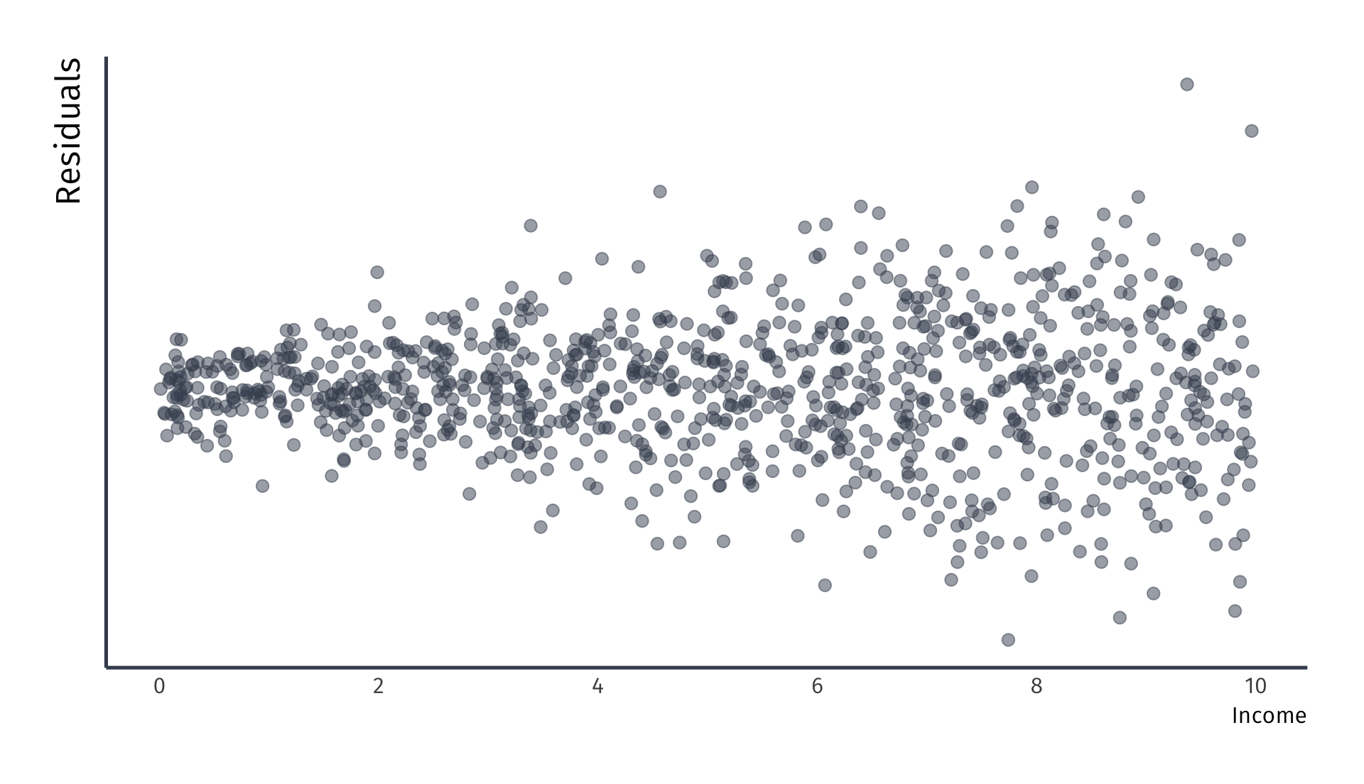
Heteroskedasticity Ex.

Suppose we study the following relationship:

\[ \text{Luxury Expenditure}_i = \beta_1 + \beta_2 \text{Income}_i + u_i \]

As income increases, variation in luxury expenditures increase

Variance of $u_i$ is likely larger for higher-income households
Plot of the residuals against the household income would likely reveal a funnel-shaped pattern

Common test for heteroskedasticity… Plot the residuals across $X$

There is more to be said about homo/heteroskedasticity in EC 421

Classical Assumptions of OLS

A1. Linearity: The population relationship is linear in parameters with an additive error term.

A2. Sample Variation: There is variation in $X$.

A3. Exogeniety: The $X$ variable is exogenous

A4. Homoskedasticity: The error term has the same variance for each value of the independent variable

A5. Non-autocorrelation: The values of error terms have independent distributions

Non-Autocorrelation

The values of error terms have independent distributions¹

\[ E[u_i u_j]=0, \forall i \text{ s.t. } i \neq j \]

Or…

\[ \begin{align*} \mathop{\text{Cov}}(u_i, u_j) &= E[(u_i - \mu_u)(u_j - \mu_u)]\\ &= E[u_i u_j] = E[u_i] E[u_j] = 0, \text{where } i \neq j \end{align*} \]

Non-Autocorrelation

The values of error terms have independent distributions

\[ E[u_i u_j]=0, \forall i \text{ s.t. } i \neq j \]

Implies no systematic association between pairs of individual $u_i$
Almost always some unobserved correlation across individuals¹
Referred to as clustering problem.
An easy solution exists where we can adjust our standard errors

Let’s take a moment to talk about the variance of the OLS estimator

Proof of the population variance

By definition

\[ Var(\hat{\beta}_2) = E\left[\left(\hat{\beta}_2 - E(\hat{\beta}_2)\right)^2\right] = E\left[\left(\hat{\beta}_2 - \beta_2\right)^2\right] \]

Step 1: Derive an expression for $\hat{\beta}_2 - \beta_2$:

\[ \hat{\beta}_2 - \beta_2 = \frac{\sum(y_i - \bar{y})(x_i - \bar{x})}{\sum(x_i - \bar{x})^2} - \beta_2 \]

Substitute for $Y_i$:

\[ \hat{\beta}_2 - \beta_2 = \frac{\sum((\beta_1 + \beta_2x_i + u_i) - \bar{y})(x_i - \bar{x})}{\sum(x_i - \bar{x})^2} - \beta_2 \]

Proof of the population variance

Substitute $\bar{y} = \beta_1 + \beta_2\bar{x}$:

\[ \hat{\beta}_2 - \beta_2 = \frac{\sum(u_i(x_i - \bar{x}))}{\sum(x_i - \bar{x})^2} \]

Step 1: Take variance $\hat{\beta}_2 - \beta_2$:

\[ Var(\hat{\beta}_2) = E\left[\left(\frac{\sum(u_i(x_i - \bar{x}))}{\sum(x_i - \bar{x})^2}\right)^2\right] \]

Square the numerator:

\[ Var(\hat{\beta}_2) = E\left[\frac{\sum(u_i(x_i - \bar{x}))\sum(\epsilon_j(x_j - \bar{x}))}{\left(\sum(x_i - \bar{x})^2\right)^2}\right] \]

Using A5, we can simplify:

\[ Var(\hat{\beta}_2) = \frac{1}{\left(\sum(x_i - \bar{x})^2\right)^2}\sum E(u_i^2(x_i - \bar{x})^2) \]

Using A4: $Var(u_i) = \sigma^2$.

\[ Var(\hat{\beta}_2) = \frac{\sigma^2}{\left(\sum(x_i - \bar{x})^2\right)^2}\sum (x_i - \bar{x})^2 \]

Thus we arrive at the variance of the OLS slope parameter:

\[ Var(\hat{\beta}_2) = \frac{\sigma^2}{\sum(x_i - \bar{x})^2} \]

If A4. and A5. are satisfied, along with A1., A2., and A3., then we are using the most efficient linear estimator.

Classical Assumptions of OLS

A1. Linearity: The population relationship is linear in parameters with an additive error term.

A2. Sample Variation: There is variation in $X$.

A3. Exogeniety: The $X$ variable is exogenous

A4. Homoskedasticity: The error term has the same variance for each value of the independent variable

A5. Non-autocorrelation: The values of error terms have independent distributions

A6. Normality: The population error term in normally distributed with mean zero and variance $\sigma^2$

Nomality (A6.)

The population error term in normally distributed with mean zero and variance $\sigma^2$

Or,

\[ u \sim N(0,\sigma^2) \]

Where $\sim$ stands for distributed by and $N$ stands for normal distribution

However, A6. is note required for efficientcy nor unbiasedness

Gauss Markov

Gauss-Markov Theorem

OLS is the Best Linear Unbiased Estimator (BLUE) when the following assumptions hold:

A1. Linearity: The population relationship is linear in parameters with an additive error term.

A2. Sample Variation: There is variation in $X$.

A3. Exogeniety: The $X$ variable is exogenous

A4. Homoskedasticity: The error term has the same variance for each value of the independent variable

A5. Non-autocorrelation: The values of error terms have independent distributions

Gauss-Markov Theorem

OLS is the Best Unbiased Estimator (BUE) when the following assumptions hold:

A1. Linearity: The population relationship is linear in parameters with an additive error term.

A2. Sample Variation: There is variation in $X$.

A3. Exogeniety: The $X$ variable is exogenous

A4. Homoskedasticity: The error term has the same variance for each value of the independent variable

A5. Non-autocorrelation: The values of error terms have independent distributions

A6. Normality: The population error term in normally distributed with mean zero and variance $\sigma^2$

Population vs. sample, revisited

Population vs. Sample

Q: Why do we care about population vs. sample?

\[ \begin{align*} y_i &= 2.53 + 0.57 x_i + u_i \\ \end{align*} \]

Population vs. Sample

Q: Why do we care about population vs. sample?

\[ \begin{align*} y_i &= 2.53 + 0.57 x_i + u_i \\ \hat{y}_i &= 2.36 + 0.61 x_i \end{align*} \]

Population vs. Sample

Q: Why do we care about population vs. sample?

$$ \[\begin{align*} y_i &= 2.53 + 0.57 x_i + u_i \\ \hat{y}_i &= 2.79 + 0.56 x_i \end{align*}\] $$

Population vs. Sample

Q: Why do we care about population vs. sample?

\[ \begin{align*} y_i &= 2.53 + 0.57 x_i + u_i \\ \hat{y}_i = 3.21 + 0.45 x_i \end{align*} \]

By now you should know where this is going… Repeat 10,000 times

Population vs. Sample

Q: Why do we care about population vs. sample?

On average, the regression lines match the population line nicely.
However, individual lines (samples) can miss the mark.

Answer: Uncertainty matters.

This sampling variation creates uncertainty.
$\hat{\beta}_1$ and $\hat{\beta}_2$ are random variables that depend on the random sample.

OLS Variance

Variance of the slope estimator:

\[ \mathop{\mathrm{Var}}(\hat{\beta}_2) = \frac{\sigma^2}{\sum_{i=1}^n (X_i - \bar{X})^2} \]

As error variance increases, variance of the slope estimator increases
As variation in $X$ increases, variance of the slope estimator decreases
Larger sample sizes exhibit more variation in $X \implies \mathop{\mathrm{Var}}(\hat{\beta}_2)$ falls as $n$ rises.

OLS Variance

Variance of the slope estimator:

\[ \mathop{\mathrm{Var}}(\hat{\beta}_2) = \frac{\sigma^2}{\sum_{i=1}^n (X_i - \bar{X})^2} \]

As error variance increases, variance of the slope estimator increases
As variation in $X$ increases, variance of the slope estimator decreases
Larger sample sizes exhibit more variation in $X \implies \mathop{\mathrm{Var}}(\hat{\beta}_2)$ falls as $n$ rises.

Same as before $u_i \sim (0,1)$, $X_i \sim (0,1.5)$, $n = 30$

Increase variance in error term $u_i \sim (0,2.5)$, $X_i \sim (0,1.5)$, $n = 30$

OLS Variance

Variance of the slope estimator:

\[ \mathop{\mathrm{Var}}(\hat{\beta}_2) = \frac{\sigma^2}{\sum_{i=1}^n (X_i - \bar{X})^2} \]

As error variance increases, variance of the slope estimator increases
As variation in $X$ increases, variance of the slope estimator decreases
Larger sample sizes exhibit more variation in $X \implies \mathop{\mathrm{Var}}(\hat{\beta}_2)$ falls as $n$ rises.

Original simulation $u_i \sim (0,1)$, $X_i \sim (0,1.5)$, $n = 30$

Increase variance in $X_i$ term $u_i \sim (0,1)$, $X_i \sim (0,3)$, $n = 30$

OLS Variance

Variance of the slope estimator:

\[ \mathop{\mathrm{Var}}(\hat{\beta}_2) = \frac{\sigma^2}{\sum_{i=1}^n (X_i - \bar{X})^2} \]

As error variance increases, variance of the slope estimator increases
As variation in $X$ increases, variance of the slope estimator decreases
Larger sample sizes exhibit more variation in $X \implies \mathop{\mathrm{Var}}(\hat{\beta}_2)$ falls as $n$ rises.

Original simulation $u_i \sim (0,1)$, $X_i \sim (0,1.5)$, $n = 30$

Increase sample size ($n$) in $X_i$ term $u_i \sim (0,1)$, $X_i \sim (0,1)$, $n = 60$

We will further this discussion next time to conduct inference.